![]()
With the release of Servidor Couchbase version 6.0 Beta, the Couchbase Analytics Service (CBAS) officially takes another step toward general availability.
We used an earlier preview release for the Couchbase Connect Silicon Valley technical demonstration. This post will dive into the details, including looking at the code and queries used.
You can see a video of the demonstration (forwarded to the analytics part) here.
What is CBAS and how does it compare to “standard” Couchbase?
Whereas with an operational database you typically perform optimized, predefined queries with supporting indexes, CBAS is designed to efficiently execute complex, often ad hoc queries over large datasets. By adding CBAS as a separate, independently scalable service, o Plataforma de dados Couchbase can handle heavy analytics work without impacting operational throughput.
For an in-depth introduction to the Couchbase Analytics Service, click on this link.
Example Data and Configuration
We created over 100 million documents of synthesized medical data based on the FHIR standard for use in the demonstration. Real deployments of course often reach into terabytes of data. The size of this set meant we still had to face realistic issues with optimization.
Configuring CBAS for this application is quite easy. You can find full instructions for setting up the demo in esta postagem do blog e este vídeo. There’s a smaller dataset provided in the Repositório do GitHub for the project.
For the analytics piece specifically, we just need to create a bucket, and designate a few shadow datasets. Interoperation gets kicked off by the final “CONNECT” command. These are all executed in the analytics query engine. (Note this is different from N1QL. If using the admin console, you must run these in the analytics section.)
(Importante: These commands work as of Couchbase 6.0.0 Beta. For updates and information on breaking changes in other versions, please refer to Changes to the Couchbase Analytics Service.)
|
1 2 3 4 |
CRIAR DATASET patient ON health ONDE resourceType = "Patient" CRIAR DATASET condition ON health ONDE resourceType = "Condição" CRIAR DATASET encounter ON health ONDE resourceType = "Encounter" CONNECT LINK Local |
Notice there’s no ETL involved. Of course other business concerns might require conditioning the data in some way, but having an integrated platform can save a lot of tooling headaches.
Code and Queries
Web Client
The front end UI code is in web/client/src/components/views/Analytics.vue. It has some selectors to parametrize the queries, and some visualization components for the results.
We visualize the data two ways. One uses a line graph to show aggregate values. (We use Chart.js for this.) The graph is interactive. Clicking on an aggregate point brings up a table with details. We won’t go into more detail here. Most of the work is done on the server side. The information gets prepared there in a way that’s easily consumed by the client.
Web Server and Queries
The data is retrieved via REST endpoints written in Node.js. As with the other REST endpoints, the Node server-side code mostly wraps queries to the database.
We chose to organize this via four endpoints: analyticsByAge, analyticsByAgeDetails, analyticsSociale analyticsSocialDetails.
The code for a grouping (age, social media) is similar. Let’s take a look at analyticsByAge. The code is in web/server/controllers/searchController.js.
|
1 2 3 4 5 6 7 8 9 10 11 12 13 14 15 16 17 18 19 20 21 22 23 24 25 26 27 28 29 30 31 32 33 34 35 36 37 38 39 40 41 42 43 44 45 46 47 48 49 50 51 52 53 54 55 56 57 58 59 60 61 62 63 64 65 66 67 68 69 70 71 72 73 74 75 76 77 78 79 80 81 82 83 84 85 86 87 88 |
var expresso = exigir("expresso); var randomHexColor = exigir('random-hex-color'); var router = expresso.Router(); // Based on Couchbase colors (TM) const palette = [ '#E72731', '#0074e0', '#f0ce0f', '#b26cda', '#00b6bd', '#00a1db', '#eb242a', '#fd9d0d' ]; const searchKeyAllGenders = 'All Genders'; const searchKeyAllCities = 'All Cities'; ... exportações.analyticsByAge = assíncrono função(req, res, próxima) { deixar couchbase = req.aplicativo.locais.couchbase; deixar agrupamento = req.aplicativo.locais.agrupamento; deixar CbasQuery = couchbase.CbasQuery; deixar consulta = `SELECIONAR year_month, age_group, count(p.id) como patient_count DE condition c, patient p ONDE substring_after(c.assunto.reference, "uuid:") /*+ indexnl */ = meta(p).id E c.código.texto = '${req.query.diagnosis}' E data(c.assertedDate) > data('2007-10-01') `; se (!searchAllGenders(req.consulta.gender)) { consulta += `E p.gender = '${req.query.gender.toLowerCase()}' `; } se (!searchAllCities(req.consulta.cidade)) { consulta += `E p.endereço[0].cidade = '${req.query.city}' `; } consulta += `GRUPO BY substring(c.assertedDate, 0, 7) como year_month, to_bigint((get_year(current_date()) - get_year(data(p.birthDate))) / 30) como age_group ORDEM BY year_month` consulta = CbasQuery.fromString(consulta); agrupamento.consulta(consulta, (erro, resultado) => { se (erro) { retorno res.status(500).enviar({ código: erro.código, mensagem: erro.mensagem }); } deixar grupos = [0, 1, 2, 3]; deixar stats = {}; deixar datasets = []; deixar rótulos = []; grupos.forEach(grupo => stats[grupo] = {}); para (const registro de resultado) { se (!stats[registro.age_group]) stats[registro.age_group] = {}; se (!rótulos.includes(registro.year_month)) { rótulos.empurrar(registro.year_month); grupos.forEach(grupo => stats[grupo][registro.year_month] = 0); } stats[registro.age_group][registro.year_month] += registro.patient_count; } deixar knife = 0; para (const chave em stats) { se (stats.hasOwnProperty(chave)) { var entradas = []; para (deixar nn = 0; nn < rótulos.comprimento; ++nn) { entradas.empurrar(stats[chave][rótulos[nn]]); } datasets.empurrar({ dados: entradas, rótulo: `${30*chave} - ${30*chave + 29}`, fill: falso, backgroundColor: 'rgba(0, 0, 0, 0)', borderColor: palette[knife], pointBackgroundColor: palette[knife] }); } knife = (knife + 1) % palette.comprimento; } res.enviar({ rótulos: rótulos, datasets: datasets }); }); } |
The Express setup code (in app.js) takes care of connecting to the cluster. It passes two globally shareable control objects, the couchbaseobject, which provides some general interfaces, and the agrupamentoobject, which is specific to a single cluster.
Past that, the listing above breaks down into two blocks, generating the query, then handling the results.
Querying with SQL++
CBAS uses SQL++. Developed in collaboration with UC San Diego, UC Irvine, and Couchbase, SQL++ is an advanced query language designed for the JSON format, yet is backward-compatible with SQL.
The query pulls from two document types, Conditons, and Patients. What we want to graph is the number of patients with a condition, listed by the month and year the condition started, binned by age. Walking through the query, we see we’re getting just that from the SELECIONAR cláusula.
O DE clause might seem a bit surprising. If you look back at the configuration, you’ll see we’ve set up two datasets, condition e patient. These are just analytics buckets comprising the corresponding document types.
We then have a series of selectors that are the real heart of the query. The first condition substring_after(c.subject.reference, "uuid:") /*+ indexnl */ = meta(p).id is especially interesting. This limits the results to only those documents where the subject (i.e. the patient) in the condition record matches the patient id of the patient document. In other words, it’s performing an inner join.
In CBAS, inner joins, by default, use a hash algorithm. The short sequence that looks like a comment (/*+ indexnl */) is actually a hint to the query compiler that it should try to perform an index nested loop join. This can be more efficient than a hash, but requires an index. Here, the index comes for free in the form of the document keys (document id) of the patient records.
The rest of the query does things like filter by condition, limit the data to a 10-year range, groups and orders the output, and splits it into 30-year chunks by patient age. It only deviates from regular SQL in one other place. A patient can have more than one address.
We want to filter by city, if the user chooses. We can do that directly, even though the patient addresses are kept in an array. In this case, with the snippet AND p.address[0].city = '${req.query.city}', you can see we’ve hard-coded picking the first address. Other operators give you more sophisticated ways of handling this. For example, you could generate separate results for each array entry.
Query Optimization
Optimizing queries can be critical to application success. With that in mind, I want to dive a little deeper on the join. The Couchbase admin console can display a query plan, essentially a break down of the operations the query planner maps out.
We won’t go through an entire plan. Instead, let’s take a look at the difference that hint makes. Here’s a side-by-side diff of the the same query, with and without the hint.
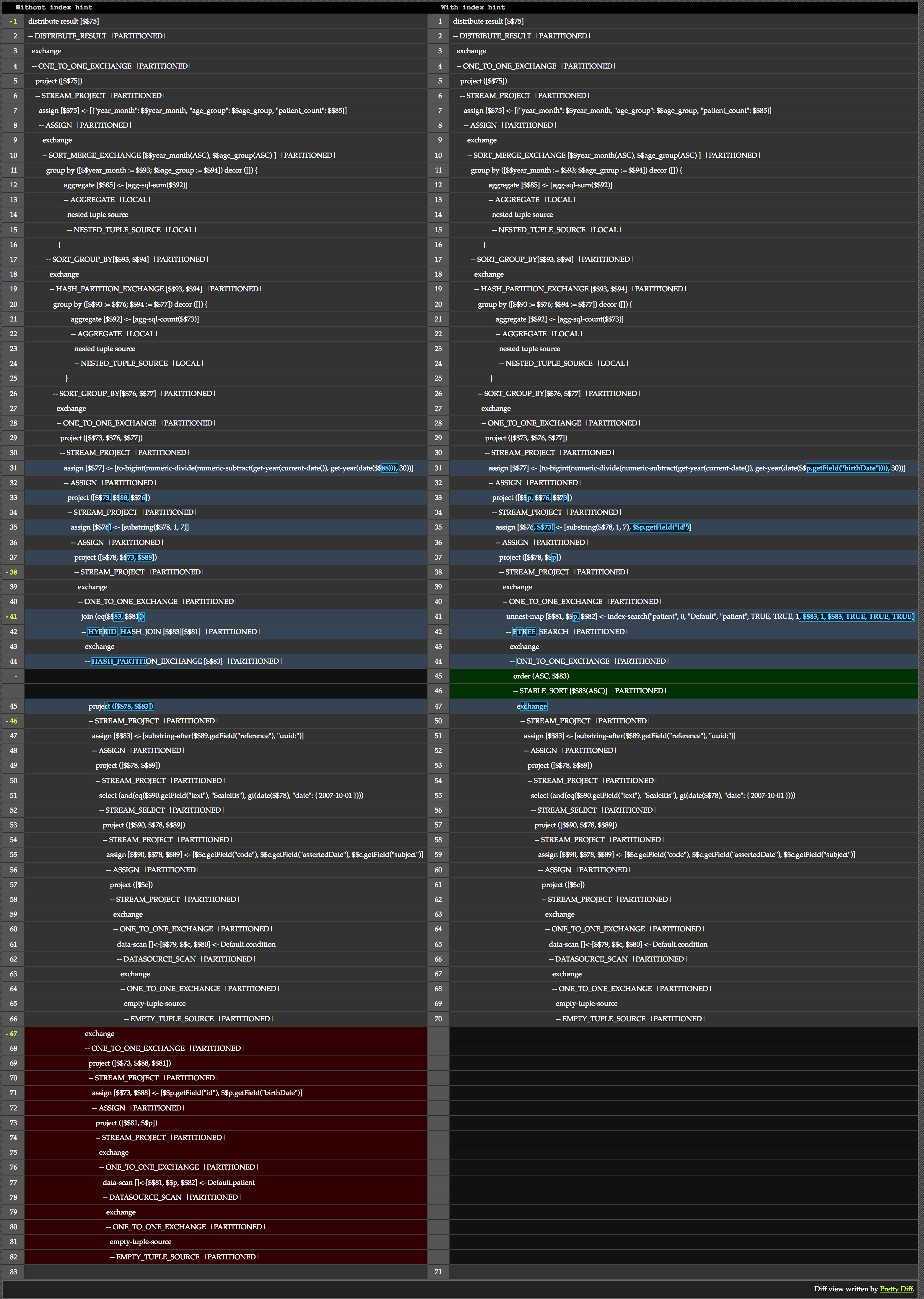
We can see the core of the difference the hint makes in lines 41-45. As promised, we can see the version without the hint uses hashing, while the one with the hint can instead use a B-tree search.
Further, we see at the bottom of the comparison the version with no hint ran extra data scans and projections to pull in the needed information.
I want to call out one other tidbit that helps me with reading these plans. Looking through you see a lot of sections referring to an troca operation. Loosely speaking, exchange operations indicate where data is partitioned up and processed in parallel. You can read more about them in esta postagem do blog. For an even more complete understanding, read section D, part 2 on connectors in the Hyracks Library aqui.
Query Results and REST Response
Once we have the complete SQL++ query as a string, we use the CbasQuery sub-object of the couchbase object to turn that into a query we can hand off to the cluster.
The code that follows manipulates the results into the form used by Chart.js. The code may look a little convoluted. That’s because we want to plot only those months where at least one patient had a diagnosis. We also have to account for results sets where the same month may have patients in different age groups. Here’s small sample of what the data looks like.
|
1 2 3 4 5 6 7 8 9 10 11 12 13 14 15 16 17 18 19 |
[ ... { "year_month": "2008-12", "age_group": 2, "patient_count": 1 }, { "year_month": "2009-02", "age_group": 0, "patient_count": 1 }, { "year_month": "2009-02", "age_group": 1, "patient_count": 3 }, ... ] |
As you can see, February of 2009 had no incidents, while January had patients that fell into two different age brackets.
Going back to the code, we see the first loop creates two data structures.
O rótulos array will give the text along the x-axis of our graph with the year and month of the onset of the condition. The code only adds entries for dates included in the result set. This may not include every month over the range spanned. (In essence, we’re removing months where no patients contracted a condition from the graph.)
O stats variable is effectively a two dimensional array that totals the number of patients for each age group and year/month of onset. This will be the actual data plotted.
Once we have the data in this form, the second loop iterates over the stats and creates the structure Chart.js expects.
Conclusão
The rest of the Analytics code and queries are all very similar to the parts we’ve examined. For further information and examples, take a look at the Analytics primer aqui. It uses sample data distributed with every version of Couchbase.
For more on this sample application, view the video of the keynote aqui, along with these other posts.
Postscript
Couchbase is open source and free to try out.
Comece a usar com sample code, example queries, tutorials, and more.
Find more resources on our developer portal.
Follow us on Twitter @CouchbaseDev.
You can post questions on our fóruns.
We actively participate on Stack Overflow.
Hit me up on Twitter with any questions, comments, topics you’d like to see, etc. @HodGreeley